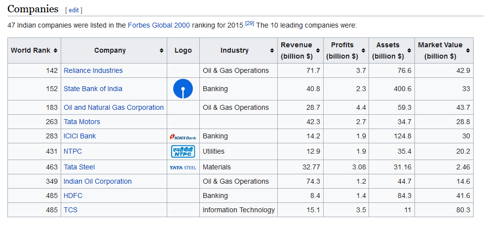
In this blog we will do web scraping using python and convert html table into pandas dataframe. After that we will also analyze the data. We will scrape data of "Economic development in India", which is available on wikipedia and url is https://en.wikipedia.org/wiki/Economic_development_in_India.

We will grab below html table from wikipedia and analyze these data using pandas and matplotlib module.


Requests is an elegant and simple HTTP library for Python, built for human beings. To install Requests, simply we can run this command in your terminal:
python -m pip install requests
Making a request with Requests is very simple. Simply we need to import the Requests module.
import requests

r = requests.get('WEB-PAGE-URL')
Now, we have a Response object called r. We can get all the information we need from this object.
import requests
page_url = "https://en.wikipedia.org/wiki/Economic_development_in_India"
We are getting webpage content using requests.get() function in that passing timeout and verify parameters.
Requests can also ignore verifying the SSL certificate if you set verify to False. By default, verify is set to True. Option verify only applies to host certs.
Most requests to external servers should have a timeout attached, in case the server is not responding in a timely manner. By default, requests do not time out unless a timeout value is set explicitly. Without a timeout, our code may hang for minutes or more.
The connect timeout is the number of seconds Requests will wait for your client to establish a connection to a remote machine call on the socket. It’s a good practice to set connect timeouts.
The timeout value will be applied to both the connect and the read timeouts. Specify a tuple if you would like to set the values separately.
html = requests.get(page_url, timeout = 5, verify = True)
html.text[:1000]
import pandas as pd
pandas.read_html
pandas.read_html(io, match='.+', flavor=None, header=None, index_col=None, skiprows=None, attrs=None, parse_dates=False, thousands=',', encoding=None, decimal='.', converters=None, na_values=None, keep_default_na=True, displayed_only=True)
Read HTML tables into a list of DataFrame objects.Parameters
io: str, path object or file-like object

    A URL, a file-like object, or a raw string containing HTML. Note that lxml only accepts the http, ftp and file url protocols. If you have a URL that starts with 'https' you might try removing the 's'.

match: str or compiled regular expression, optional

    The set of tables containing text matching this regex or string will be returned. Unless the HTML is extremely simple you will probably need to pass a non-empty string here. Defaults to ‘.+’ (match any non-empty string). The default value will return all tables contained on a page. This value is converted to a regular expression so that there is consistent behavior between Beautiful Soup and lxml.


flavor: str, optional

    The parsing engine to use. ‘bs4’ and ‘html5lib’ are synonymous with each other, they are both there for backwards compatibility. The default of None tries to use lxml to parse and if that fails it falls back on bs4 + html5lib.

header: int or list-like, optional

    The row (or list of rows for a MultiIndex) to use to make the columns headers.

index_col: int or list-like, optional

        The column (or list of columns) to use to create the index.

skiprows: int, list-like or slice, optional

    Number of rows to skip after parsing the column integer. 0-based. If a sequence of integers or a slice is given, will skip the rows indexed by that sequence. Note that a single element sequence means ‘skip the nth row’ whereas an integer means ‘skip n rows’.

attrs: dict, optional

    This is a dictionary of attributes that you can pass to use to identify the table in the HTML.

parse_dates: bool, optional

thousands: str, optional

        Separator to use to parse thousands. Defaults to ','.

encoding: str, optional

        The encoding used to decode the web page. Defaults to None.

decimalstr, default '.'

        Character to recognize as decimal point.

converters: dict, default None

        Dict of functions for converting values in certain columns. Keys can either be integers or column labels, values are functions that take one input argument, the cell (not column) content, and return the transformed content.

 na_values: iterable, default None

     Custom NA values.

 keep_default_na: bool, default True

     If na_values are specified and keep_default_na is False the default NaN values are overridden, otherwise they're appended to.

displayed_only: bool, default True

        Whether elements with "display: none" should be parsed.
Returns
    dfs

        A list of DataFrames.

See alsodfs = pd.read_html(html.text)
dfs
We can see many tables we got. We have to display second tables.
len(dfs)
I have checked index 4th provides our required data.
dfs[4].head()
df = dfs[4]
df.head()
df.shape
df.info()
df.columns
import matplotlib.pyplot as plt
plt.figure(figsize=(10,6))
plt.plot(df['Year'], df['Growth (real) (%)'])

plt.title('GDP Growth Rate in %', color = "red", fontsize = 20)
plt.xlabel("Year")
plt.ylabel("Growth (real) (%)")
plt.show()
plt.figure(figsize=(10,6))
plt.bar(df['Year'], df['Growth (real) (%)'])

plt.title('GDP Growth Rate in %', color = "red", fontsize = 20)
plt.xlabel("Year")
plt.ylabel("Growth (real) (%)")
plt.show()
plt.figure(figsize=(15,8))
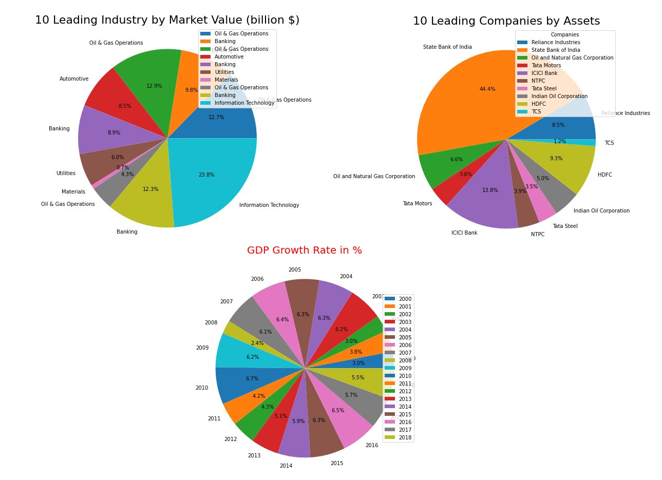
plt.pie(df['Growth (real) (%)'], labels = df['Year'], autopct='%1.1f%%')

plt.title('GDP Growth Rate in %', color = "red", fontsize = 20)
plt.legend(loc ="center right", fontsize = 10)
plt.show()
dfs[5].head()
df1 = dfs[5]
df1.head(10)
df1.shape
df1.info()
plt.figure(figsize=(12,8))
plt.bar(df1['Company'], df1['Assets (billion $)'])

plt.title('10 Leading Companies by Assets', fontsize = 20)
plt.xlabel("Companies", fontsize = 20)
plt.ylabel("Assets in billion '$'", fontsize = 20)
plt.xticks(rotation=45, ha='right')
plt.show()
plt.figure(figsize=(15,8))
plt.pie(df1['Assets (billion $)'], labels = df1['Company'], autopct='%1.1f%%')

plt.legend(title = "Companies", loc ="upper right")
plt.title('10 Leading Companies by Assets', fontsize = 22)

plt.show()
We can see, according to assets comapany "State Bank of India" is the largest one.
First need to check Industry column has NAN value or not.
df1['Industry'].isna().sum()
If we see data, company "Tata Motors" doesn't have Industry. So let add industry in that.
import numpy as np
df1['Industry'] = np.where((df1.Company == 'Tata Motors'),'Automotive', df1.Industry)
df1['Industry']
df1
plt.figure(figsize=(10,6))

plt.bar(df1['Industry'], df1['Market Value (billion $)'])

plt.title('10 Leading Industry by Market Value (billion $)', fontsize = 22)
plt.xlabel("Industry", fontsize = 20)
plt.ylabel("Market Value (billion $)", fontsize = 20)
plt.show()
plt.figure(figsize=(15,8))
plt.pie(df1['Market Value (billion $)'], labels = df1['Industry'], autopct='%1.1f%%')

plt.legend(loc ="upper right", fontsize = 10)
plt.title('10 Leading Industry by Market Value (billion $)', fontsize = 22)

plt.show()